

PhysBound
Physical Layer Linter — an MCP server that validates RF and physics calculations against hard physical limits, catching AI hallucinations in engineering workflows.






LLMs generate plausible-sounding RF numbers that violate fundamental physics — throughput above the Shannon limit, antenna gains no aperture can produce, radar ranges the range equation forbids. PhysBound gives any MCP-compatible AI assistant six validated calculation tools, backed by CODATA constants (via SciPy) and dimensional analysis (via Pint). Impossible claims return structured PhysicalViolationError responses with the violated law, the computed limit, and a LaTeX explanation — not silent failures.
| Tool | What it validates |
|---|---|
rf_link_budget | Friis link budgets: FSPL, received power, antenna gains vs. aperture/Harrington limits |
shannon_hartley | Throughput claims against channel capacity C = B log2(1 + SNR) |
noise_floor | Thermal noise kTB, Friis noise-figure cascades, receiver sensitivity |
radar_range | Detection-range claims against the monostatic radar range equation |
antenna_gain | Gain limits, beamwidth, and far-field distance for a single antenna |
radar_ambiguity | Pulse-Doppler unambiguous range/velocity, Doppler aliasing, range resolution |
Installation
PhysBound is a standard stdio MCP server published on PyPI. The recommended launch command is uvx physbound, which fetches and runs the latest release in an isolated environment — no manual install step.
First run:
uvxdownloads ~60 MB of dependencies (SciPy, NumPy) the first time. Runuvx physboundonce in a terminal to pre-cache them (Ctrl-C to exit); subsequent starts are instant.
Claude Code
claude mcp add physbound -- uvx physbound
Claude Desktop
Add to claude_desktop_config.json (macOS: ~/Library/Application Support/Claude/, Windows: %APPDATA%\Claude\):
{
  "mcpServers": {
    "physbound": {
      "command": "uvx",
      "args": ["physbound"]
    }
  }
}
Cursor, Windsurf, and other MCP clients
Use the same JSON server entry as above in your client's MCP configuration file (Cursor: ~/.cursor/mcp.json; Windsurf: ~/.codeium/windsurf/mcp_config.json).
Without uv
If you prefer a plain Python install (requires Python 3.12+):
pip install physbound
then set "command": "physbound" (with no args) in the client configuration.
Once configured, ask your assistant an RF question — "Can a 20 MHz channel with 15 dB SNR support 500 Mbps?" — and it will answer with physics-validated numbers.
Command-Line Usage
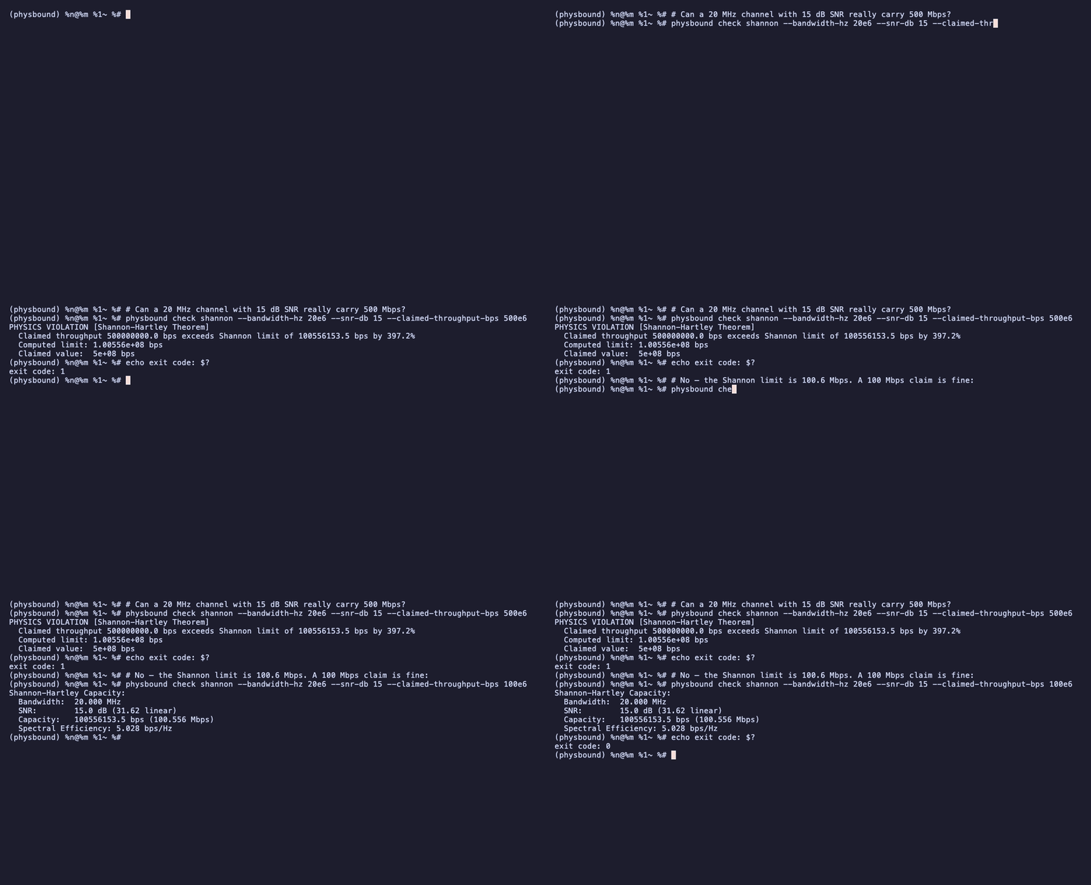
The same validators are available directly from the terminal — useful in scripts and CI pipelines, since a physics violation exits with code 1:
$ physbound check shannon --bandwidth-hz 20e6 --snr-db 15 --claimed-throughput-bps 500e6
PHYSICS VIOLATION [Shannon-Hartley Theorem]
  Claimed throughput 500000000.0 bps exceeds Shannon limit of 100556153.5 bps by 397.2%
  Computed limit: 1.00556e+08 bps
  Claimed value:  5e+08 bps
$ echo $?
1
$ physbound check shannon --bandwidth-hz 20e6 --snr-db 15 --claimed-throughput-bps 100e6
Shannon-Hartley Capacity: ...   # exit code 0
Available subcommands: check {link-budget, shannon, noise, radar-range, antenna, radar-ambiguity} (flags mirror the MCP tool parameters; add --json for the full structured result) and serve --transport {stdio,http} for running the MCP server over HTTP. See physbound check --help for details.
What LLMs Get Wrong
Sixteen real hallucination patterns, each caught by PhysBound's test suite:
| # | Category | LLM Hallucination | PhysBound Truth | Verdict |
|---|---|---|---|---|
| 1 | Shannon-Hartley | A 20 MHz 802.11n channel with 15 dB SNR can achieve 500 Mbps | Shannon limit: 100.6 Mbps (not 500 Mbps) | CAUGHT |
| 2 | Shannon-Hartley | A 100 MHz 5G channel with 20 dB SNR delivers 2 Gbps | Shannon limit: 665.8 Mbps (not 2000 Mbps) | CAUGHT |
| 3 | Antenna Aperture | A 30 cm dish antenna at 1 GHz provides 45 dBi gain | Physical limit: 12.1 dBi (Harrington); aperture eta=1: 9.9 dBi; typical dish: 7.4 dBi (eta=0.55) (not 45 dBi) | CAUGHT |
| 4 | Thermal Noise | Receiver noise floor of -180 dBm/Hz at room temperature | Thermal noise floor: -174.0 dBm/Hz at 290K (not -180 dBm/Hz) | CAUGHT |
| 5 | Link Budget / FSPL | Wi-Fi at 2.4 GHz with 20 dBm TX reaches 10 km with -40 dBm RX power | Actual RX power at 10 km: -94.1 dBm (not -40 dBm) | CAUGHT |
| 6 | Link Budget / FSPL | A 1W transmitter at 12 GHz with 0 dBi antennas reaches GEO at -80 dBm | Actual RX power at GEO: -175.1 dBm (not -80 dBm) | CAUGHT |
| 7 | Link Budget / FSPL | Bluetooth at 2.4 GHz with 0 dBm TX and 0 dBi antennas reaches 1 km at -60 dBm | Actual RX power at 1 km: -100.1 dBm (not -60 dBm) | CAUGHT |
| 8 | Shannon-Hartley | A 10 MHz LTE channel at 10 dB SNR supports 1 Gbps | Shannon limit: 34.6 Mbps (not 1000 Mbps) | CAUGHT |
| 9 | Noise Cascade | Receiver NF is the same regardless of stage order: LNA(20dB/1.5dB) + Mixer(10dB/8dB) | LNA first: 1.66 dB vs mixer first: 8.03 dB (penalty: 6.4 dB) | CAUGHT |
| 10 | Antenna Aperture | A 10 cm patch antenna at 900 MHz provides 20 dBi gain | Physical limit: 4.4 dBi (Harrington, D < lambda); aperture eta=1: -0.5 dBi; typical: -3.1 dBi (eta=0.55) (not 20 dBi) | CAUGHT |
| 11 | Radar Range Equation | Doubling transmit power doubles radar detection range | Range increases by factor 1.189 (2^(1/4) = 1.189), not 2.0 | CAUGHT |
| 12 | Radar Range Equation | Small drone (0.01 m^2 RCS) detectable at 200 km by 1 kW X-band radar with 30 dBi gain | Max range: 2.7 km for 0.01 m^2 RCS at 1 kW X-band (not 200 km) | CAUGHT |
| 13 | Antenna Gain | A 0.5 m user-terminal dish at 12 GHz gives 50 dBi gain | Physical limit: 36.1 dBi (Harrington); typical dish: 33.4 dBi (eta=0.55) (not 50 dBi) | CAUGHT |
| 14 | Antenna Gain | A 3 m dish at 10 GHz is in its far field at 10 m, so gain can be measured there | Far-field distance 2D^2/lambda = 600 m; 10 m is in the near field | CAUGHT |
| 15 | Radar Ambiguity | A 10 GHz radar at 10 kHz PRF unambiguously measures 500 m/s | v_ua = lambda*PRF/4 = +/-74.9 m/s (blind speed 149.9 m/s); 500 m/s aliases (not 500 m/s) | CAUGHT |
| 16 | Radar Ambiguity | A 10 GHz pulse-Doppler radar can unambiguously cover 150 km and +/-300 m/s at once | R_uav_ua = clambda/8 = 1.123e+06 m^2/s for any PRF; claimed 4.5e+07 m^2/s (40x too large) | CAUGHT |
Generated automatically by pytest tests/test_marketing.py -s
Tools
Full derivations, sources, and worked examples for every formula are in docs/formulas.md.
rf_link_budget
Computes a complete RF link budget using the Friis transmission equation and validates antenna gains against physical limits.
Example: "What's the received power for a 2.4 GHz link at 100 m with 20 dBm TX, 10 dBi TX gain, 3 dBi RX gain?"
Returns FSPL, received power, wavelength, and — when antenna diameters are supplied — gain limit checks. Gains above the hard bound G_max = max((pi D / lambda)^2, (ka)^2 + 2ka) (the eta = 1 aperture value, or Harrington's bound for electrically small antennas) are rejected; gains above the typical dish value (eta = 0.55) are accepted with a warning. Also warns inside the far-field distance 2D^2/lambda and rejects negative losses.
shannon_hartley
Computes Shannon-Hartley channel capacity C = B log2(1 + SNR) and validates throughput claims.
Example: "Can a 20 MHz channel with 15 dB SNR support 500 Mbps?"
Returns theoretical capacity, spectral efficiency, and whether the claim is physically possible, including the exact percentage by which a violating claim exceeds the Shannon limit.
noise_floor
Computes thermal noise power N = k_B T B, cascades noise figures through multi-stage receivers with the Friis noise formula, and calculates receiver sensitivity.
Example: "What's the noise floor for a 1 MHz receiver at 290 K with a two-stage LNA chain?"
Returns thermal noise in dBm and watts, cascaded noise figure, effective input noise temperature T_e = 290 K * (F - 1), and receiver sensitivity.
radar_range
Computes the monostatic radar range equation R_max = [P_t G^2 lambda^2 sigma / ((4pi)^3 S_min L)]^(1/4) and validates detection-range claims.
Example: "Can a 1 kW X-band radar with 30 dBi gain detect a 0.01 m^2 drone at 200 km?"
Returns maximum detection range, minimum detectable signal, wavelength, and intermediate values. Catches the common fourth-root fallacy that doubling power doubles range.
antenna_gain
Analyses a single antenna from its diameter or physical area: gain limits, beamwidth, and far-field distance, with optional validation of a claimed gain.
Example: "Can a 0.5 m dish at 12 GHz really give 50 dBi? What beamwidth should I expect?"
Returns the physical gain limit (aperture or Harrington bound, and which one governs), typical gain at the given efficiency (default 0.55), effective aperture, half-power beamwidth estimates, far-field distance 2D^2/lambda, and — for a claimed gain — the implied aperture efficiency and validity.
radar_ambiguity
Computes pulse-Doppler ambiguity limits for a given carrier frequency and PRF.
Example: "Can a 10 GHz radar at 10 kHz PRF unambiguously measure a 500 m/s target out to 150 km?"
Returns unambiguous range R_ua = c / (2 PRF), unambiguous velocity v_ua = lambda PRF / 4, blind speed, Doppler shift and apparent (aliased) velocity, range resolution (c tau / 2, or c / 2B with pulse compression), minimum range, duty cycle, and the range-Doppler dilemma invariant R_ua v_ua = c lambda / 8. Rejects range, velocity, or resolution claims the PRF or pulse cannot support.
Physics Guarantees
Every calculation is validated against hard physical limits:
- Speed of light:
c = 299,792,458 m/s— no exceptions - Thermal noise floor:
N = -174 dBm/Hzat 290 K — the IEEE standard reference - Shannon limit:
C = B log2(1 + SNR)— no throughput claim exceeds this - Antenna gain limit:
G_max = max((pi D / lambda)^2, (ka)^2 + 2ka)— the eta = 1 aperture value for planar apertures and Harrington's bound for any antenna in a sphere of diameter D; eta = 0.55 is a warning threshold, not a limit - Radar range equation:
R_max = [P_t G^2 lambda^2 sigma / ((4pi)^3 S_min)]^(1/4)— range obeys the fourth-root law - Receiver sensitivity:
S_min = k (T_A + T_0 (F - 1)) B * SNRwithT_e = T_0 (F - 1)referenced to 290 K - Unambiguous range:
R_ua = c / (2 PRF)— echoes beyond it fold into a later pulse interval - Unambiguous velocity:
v_ua = lambda PRF / 4— Doppler is sampled at the PRF, so|f_d| <= PRF/2 - Range-Doppler dilemma:
R_ua * v_ua = c lambda / 8— no PRF choice beats it for a given carrier
Violations return structured PhysicalViolationError responses with LaTeX explanations, not silent failures.
Examples and Documentation
- Catching Hallucinations — walkthrough of five real LLM failure modes with full JSON responses
- Interactive Demo Notebook — Jupyter notebook calling the physics engines directly
- Formula Reference — every formula, constant, and validation guard with sources
- Changelog — release history
Development
Requires uv and Python 3.12+ (CI covers 3.12–3.14):
# Clone and install
git clone https://github.com/JonesRobM/physbound.git
cd physbound
uv sync --all-extras

# Run checks
uv run pytest tests/ -v
uv run ruff check src/ tests/
uv run mypy src/physbound/

# Regenerate the hallucination table above
uv run pytest tests/test_marketing.py -s

# Start the MCP server locally
uv run physbound
Contributions that expand the set of validated physics domains are welcome — see CONTRIBUTING.md for the architecture guide and the step-by-step recipe for adding a new validator.
Use Cases
- RF system design review — validate link budgets, receiver sensitivity, and noise cascades
- Telecom proposal vetting — catch impossible throughput claims before they reach a customer
- Radar system sizing — sanity-check detection range, PRF selection, and ambiguity trade-offs
- Educational tools — teach Shannon-Hartley, Friis transmission, and thermal noise with verified calculations
- CI/CD for physics — integrate as a validation step in engineering pipelines
Support
If PhysBound is useful in your work, consider buying me a coffee.
License
MIT License. See LICENSE.
Related
- Model Context Protocol — the open standard for AI tool integration
- MCP Server Registry — official directory of MCP servers
- FastMCP — Python framework for building MCP servers