Math-Physics-ML MCP System

GPU-accelerated Model Context Protocol servers for computational mathematics, physics simulations, and machine learning.

📚 Documentation

View Full Documentation →

Guide	Description
Installation	Setup instructions for pip, uv, and uvx
Configuration	Claude Desktop & Claude Code setup
Quick Start	Get running in 5 minutes
API Reference	Complete tool documentation
Visual Demos	Interactive physics simulations

About

This system enables AI assistants to perform real scientific computing — from solving differential equations to running molecular dynamics simulations.

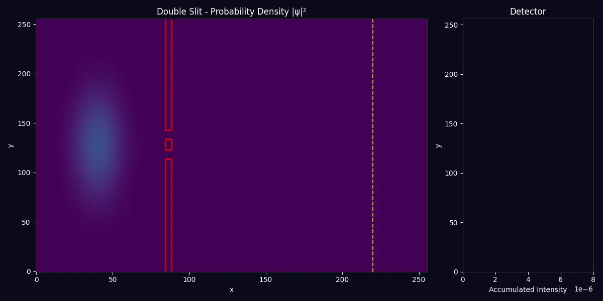
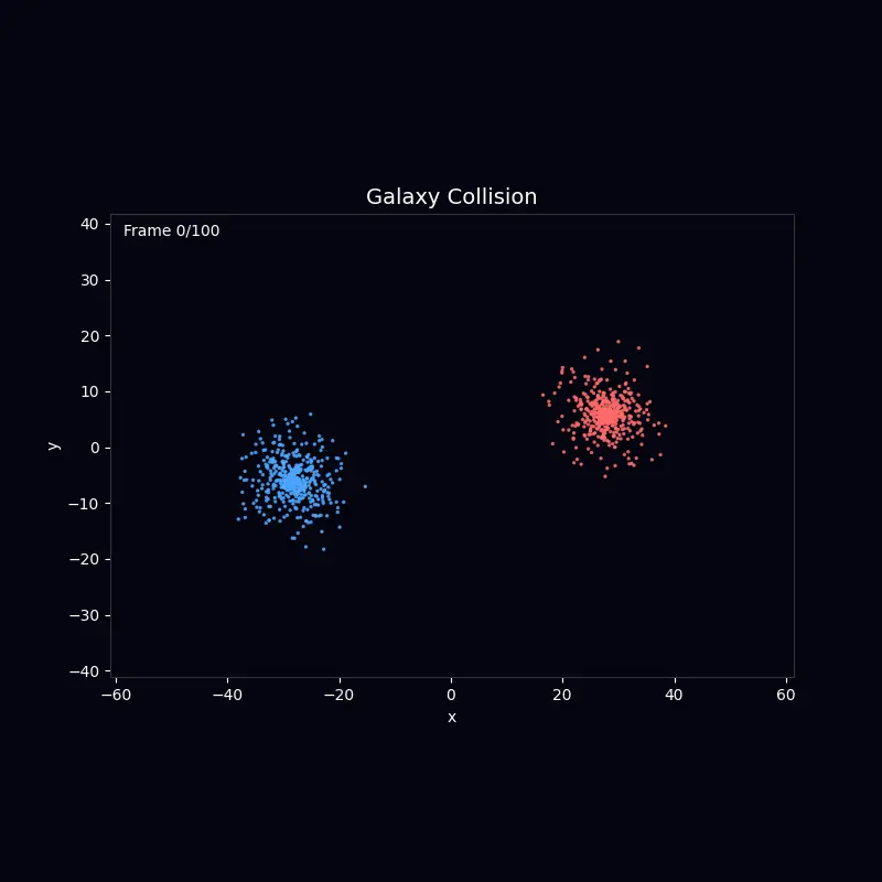
$Double-Slit Interference$ Quantum Wave Mechanics _{Double-slit interference pattern from solving the time-dependent Schrödinger equation}	$Galaxy Collision$ N-Body Dynamics _{Galaxy merger simulation using gravitational N-body calculations}
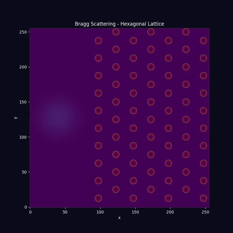
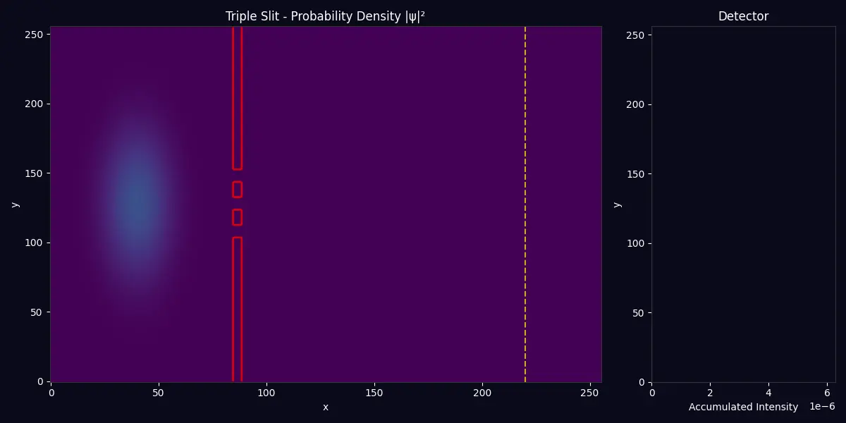
$Bragg Scattering$ Crystal Diffraction _{Bragg scattering from a hexagonal (graphene-like) lattice}	$Triple-Slit$ Multi-Slit Interference _{Complex interference patterns from three coherent sources}

Overview

This system provides 4 specialized MCP servers that bring scientific computing capabilities to AI assistants like Claude:

Server	Description	Tools
Math MCP	Symbolic algebra (SymPy) + numerical computing	14
Quantum MCP	Wave mechanics & Schrodinger simulations	12
Molecular MCP	Classical molecular dynamics	15
Neural MCP	Neural network training & evaluation	16

Key Features:

GPU acceleration with automatic CUDA detection (10-100x speedup)
Async task support for long-running simulations
Cross-MCP workflows via URI-based data sharing
Progressive discovery for efficient tool exploration

Quick Start

Installation with uvx (Recommended)

Run any MCP server directly without installation:

bash

# Run individual servers
uvx scicomp-math-mcp
uvx scicomp-quantum-mcp
uvx scicomp-molecular-mcp
uvx scicomp-neural-mcp

Installation with pip/uv

bash

# Install individual servers
pip install scicomp-math-mcp
pip install scicomp-quantum-mcp
pip install scicomp-molecular-mcp
pip install scicomp-neural-mcp

# Or install all at once
pip install scicomp-math-mcp scicomp-quantum-mcp scicomp-molecular-mcp scicomp-neural-mcp

# With GPU support (requires CUDA)
pip install scicomp-math-mcp[gpu] scicomp-quantum-mcp[gpu] scicomp-molecular-mcp[gpu] scicomp-neural-mcp[gpu]

Configuration

Claude Desktop

Add to your Claude Desktop configuration file:

macOS: ~/Library/Application Support/Claude/claude_desktop_config.json Windows: %APPDATA%\Claude\claude_desktop_config.json

json

{
  "mcpServers": {
    "math-mcp": {
      "command": "uvx",
      "args": ["scicomp-math-mcp"]
    },
    "quantum-mcp": {
      "command": "uvx",
      "args": ["scicomp-quantum-mcp"]
    },
    "molecular-mcp": {
      "command": "uvx",
      "args": ["scicomp-molecular-mcp"]
    },
    "neural-mcp": {
      "command": "uvx",
      "args": ["scicomp-neural-mcp"]
    }
  }
}

Claude Code

Add to your project's .mcp.json:

json

{
  "mcpServers": {
    "math-mcp": {
      "command": "uvx",
      "args": ["scicomp-math-mcp"]
    },
    "quantum-mcp": {
      "command": "uvx",
      "args": ["scicomp-quantum-mcp"]
    }
  }
}

Or configure globally in ~/.claude/settings.json.

Usage Examples

Math MCP

python

# Solve equations symbolically
symbolic_solve(equations="x**3 - 6*x**2 + 11*x - 6")
# Result: [1, 2, 3]

# Compute derivatives
symbolic_diff(expression="sin(x)*exp(-x**2)", variable="x")
# Result: cos(x)*exp(-x**2) - 2*x*sin(x)*exp(-x**2)

# GPU-accelerated matrix operations
result = matrix_multiply(a=matrix_a, b=matrix_b, use_gpu=True)

Quantum MCP

python

# Create a Gaussian wave packet
psi = create_gaussian_wavepacket(
    grid_size=[256],
    position=[64],
    momentum=[2.0],
    width=5.0
)

# Solve time-dependent Schrodinger equation
simulation = solve_schrodinger(
    potential=barrier_potential,
    initial_state=psi,
    time_steps=1000,
    dt=0.1,
    use_gpu=True
)

Molecular MCP

python

# Create particle system
system = create_particles(
    n_particles=1000,
    box_size=[20, 20, 20],
    temperature=1.5
)

# Add Lennard-Jones potential
add_potential(system_id=system, potential_type="lennard_jones")

# Run MD simulation
trajectory = run_nvt(system_id=system, n_steps=100000, temperature=1.0)

# Analyze diffusion
msd = compute_msd(trajectory_id=trajectory)

Neural MCP

python

# Define model
model = define_model(architecture="resnet18", num_classes=10, pretrained=True)

# Load dataset
dataset = load_dataset(dataset_name="CIFAR10", split="train")

# Train
experiment = train_model(
    model_id=model,
    dataset_id=dataset,
    epochs=50,
    batch_size=128,
    use_gpu=True
)

# Export for deployment
export_model(model_id=model, format="onnx", output_path="model.onnx")

Development

bash

# Clone the repository
git clone https://github.com/andylbrummer/math-mcp.git
cd math-mcp

# Install dependencies
uv sync --all-extras

# Install MCP servers in editable mode (required for entry points)
uv pip install --python .venv/bin/python \
  -e servers/math-mcp \
  -e servers/quantum-mcp \
  -e servers/molecular-mcp \
  -e servers/neural-mcp

# Run tests
uv run pytest -m "not gpu"  # CPU only
uv run pytest               # All tests (requires CUDA)

# Run with coverage
uv run pytest --cov=shared --cov=servers

Note: The editable install step is required because uv sync doesn't install entry point scripts for workspace packages. After this step, you can run servers directly with uv run scicomp-math-mcp.

See CONTRIBUTING.md for development guidelines.

Performance

GPU acceleration provides significant speedups for compute-intensive operations:

MCP	Operation	CPU	GPU	Speedup
Math	Matrix multiply (4096x4096)	2.1s	35ms	60x
Quantum	2D Schrodinger (512x512, 1000 steps)	2h	2min	60x
Molecular	MD (100k particles, 10k steps)	1h	30s	120x
Neural	ResNet18 training (1 epoch)	45min	30s	90x