Kshana PNT-resilience simulator
Run the validated Kshana PNT-resilience simulator (orbits, frames, GNSS, fusion) from an AI agent.
Runs on your machine from its package; the steps are below.
What it does
- Reads
- Writes
- High impact
At most: creates or changes data: records, files, settings.
What it costs
FreeOdel charges nothing per call. The publisher may charge for its own service.
Runs locally over stdio
This server isn't hosted — your MCP client launches it from a package registry. Use one of the commands below, or drop the config into your client (e.g. Claude Desktop).
Run
docker run -i --rm ghcr.io/ashfordeou/kshana-mcp:0.34.1
MCP client config
{
  "mcpServers": {
    "kshana-pnt-resilience-simulator": {
      "command": "docker",
      "args": [
        "run",
        "-i",
        "--rm",
        "ghcr.io/ashfordeou/kshana-mcp:0.34.1"
      ]
    }
  }
}

Kshana · क्षण · the precise instant
An open-source simulator for PNT (positioning, navigation and timing) resilience.










Open Kshana Studio · Install · Capabilities · Evidence · Research · Documentation · Cite

Rehearse the minute GNSS goes dark
Kshana replays jamming, spoofing and clock holdover when GNSS (Global Navigation Satellite System) signals fail, and tells you how long a system keeps time and position inside its budget, and which clock or sensor buys the most margin. It is one Rust engine. It runs in a terminal, a notebook, an IDE (integrated development environment), an AI (artificial intelligence) assistant, or in your browser.
Every run is reproducible bit for bit from the scenario, the seed and the engine version. Every capability carries one of three labels in a machine-checked ledger: VALIDATED (an independent external oracle agrees), MODELLED (internally consistent, and said out loud) or PARTNER (a hardware partner owns it).
Status: v0.34.1. A validated, reproducible simulation substrate for PNT resilience. Timing and holdover come first, because that domain is the best validated. Kshana is a study and trade-off instrument: not radio-frequency (RF) signal-generator hardware (it drives no radio and transmits nothing; its signal-level output is baseband IQ sample files for software receivers), not a hardware or certified GNSS receiver (its software receiver is an analysis tool) and not a flight product. New to the field? Start with the plain-language primer and the glossary.
Kshana Studio
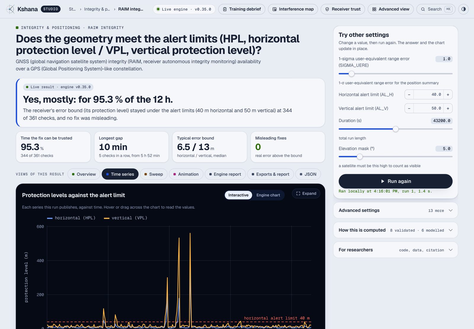
Open kshana.dev/studio and the whole engine runs in your browser, compiled to WebAssembly. Nothing to install, and nothing is uploaded. The Studio has two views of the same engine, and a switch in the header moves between them, keeping the scenario, the view and any settings you changed.
The Simple view is where the Studio opens. It starts from questions (how many satellites can I see, can I trust my position fix, how long can a clock keep time, what does a jammer do to my receiver) and from a map of everything the engine can do, each area with its share of validated methods. Open a scenario and the answer comes first: one plain sentence, written for what that scenario measures, then its key figures and a chart. At most five settings are on show, the ones that change the answer most; the rest wait under Advanced settings. How this is computed explains the method, and For researchers gives the engine's own figures, the scenario file, the code to run it from Python and the citation.

The Advanced view is the full dashboard: the scenario library, five numbered steps (Choose, Set, Run, Read results, Share or export), the key figures with PASS and FAIL chips where the run states a threshold, and every panel: overview, charts, maps, replay, the engine's report and exports. One search box reaches scenarios, domains and the fields inside them, and you can pin up to four runs and compare them side by side.
The Simple view's opening screen, and the Advanced view after a run


The Studio's source and its build notes are in web/README.md.
The site
The rest of kshana.dev is built from this repository's own files and engine runs: missions, capabilities, the evidence ledger, the published research and the editions.

Capabilities
One engine covers the whole failure chain, from the first jammed satellite to the last
nanosecond of clock holdover. The engine has 75 scenario kinds; kshana kinds lists
them and docs/SCENARIOS.md documents every field.
| Capability | What it answers |
|---|---|
| Spectrum | how a jammer takes the GNSS L band, band by band, second by second |
| Clocks and timing | how long each clock holds time after GNSS is lost |
| Constellations around any body | coverage, dilution of precision and availability around the Earth, the Moon or Mars |
| Solar system | where every planet is, and the light time of any link |
| Low-Earth-orbit navigation | a pass, a link, a navigation message and a fused fix, stage by stage |
| Campaigns | a chained mission, a sweep or a Monte Carlo ensemble in one scenario |
| Animation | a run's time series as an animated drawing, a player or frames |
| Reports | every figure with its unit and its label, in HTML (HyperText Markup Language) and JSON (JavaScript Object Notation) |
| Interoperability exports | orbits and geometry for other tools: SP3, CCSDS OMM and OEM, CZML, KML, GeoJSON, STK and SigMF |
The export formats in full: SP3 is Standard Product 3; CCSDS OMM and OEM are the Orbit Mean-elements and Orbit Ephemeris Messages of the Consultative Committee for Space Data Systems; CZML and KML are the Cesium and Keyhole Markup Languages; STK is Systems Tool Kit; SigMF is the Signal Metadata Format.

Each capability, drawn from a real run: the L-band waterfall, the coverage map, the solar system and a low-Earth-orbit pass


Run any of them with kshana example <scenario> > s.toml && kshana s.toml: the scenarios
are l-band-waterfall-jamming, constellation-multi-gnss-coverage, solar-system-tour
and leo-pass-iridium.
The full capability table, domain by domain
The full domain-by-domain detail follows; for a per-capability maturity ledger see
docs/CAPABILITY.md and docs/VALIDATION.md.
| Domain | Capability |
|---|---|
| Orbit & geometry | SGP4/SDP4 propagation (validated to 4.12 mm against all 666 AIAA 2006-6753 vectors); real two-line elements (a committed, date-stamped Celestrak gps-ops snapshot) or synthetic Walker-delta constellations whose mean elements realise the i:T/P/F formula to under 1 km over a 24 h propagation; multi-constellation visibility, dilution of precision — geometric, position, horizontal, vertical and time (GDOP/PDOP/HDOP/VDOP/TDOP), validated to 1e-6 against gnss_lib_py 1.0.4, Stanford NAV Lab (Navigation and Autonomous Vehicles Laboratory), and GNSS availability; a gradient-free constellation-design optimiser, streets-of-coverage minimum-satellite sizing, a multi-constellation comparison tool, and a Walker design sweep that tabulates coverage / PDOP / revisit-time over a planes × satellites grid and reports the Pareto-optimal designs. |
| Numerical propagator | A Cowell numerical propagator (src/propagator.rs) complementing the analytic SGP4/SDP4 path, with a hierarchical seven-perturbation force model (src/forces.rs): two-body + the full J2–J6 zonal field (the Earth-oblateness zonal harmonic coefficients J2 to J6; the exact analytic gradient of its disturbing potential), an optional EGM2008 tesseral spherical-harmonic geopotential to degree/order 70 (Earth Gravitational Model 2008; src/gravity_sh.rs; real NGA — US (United States) National Geospatial-Intelligence Agency — coefficients, Holmes–Featherstone normalized-Legendre recurrence, cross-checked against the closed-form Legendre functions and the analytic ∇V identity), epoch-driven Sun and Moon third-body gravity (a built-in low-precision ephemeris, no DE/SPK — Development Ephemeris / SPICE Spacecraft and Planet Kernel — kernel), solar-radiation pressure (cannonball model with a conical umbra+penumbra shadow), atmospheric drag (Vallado piecewise-exponential density, co-rotating atmosphere), the post-Newtonian Schwarzschild relativistic correction, and the Lense–Thirring frame-dragging term (IERS — International Earth Rotation and Reference Systems Service — Conventions 2010 §10, linear in Earth's angular momentum, ~1–2 orders below Schwarzschild) — driven by a choice of two adaptive integrators (RK4 — fourth-order Runge–Kutta — step-doubling or the Dormand–Prince RK5(4) embedded pair). Validated against Orekit 12.2 (CS GROUP, Apache-2.0) NumericalPropagator/DormandPrince853 — 275 epochs across LEO (low Earth orbit) + GTO (geostationary transfer orbit), the conservative-force tiers agreeing to a worst-case |Δr| 0.08 m over 24 h (tests/numerical_cowell_propagator_reference.rs); the atmospheric-drag tier is characterised separately (≈ 333 m / 24 h) and the absolute Sun/Moon-ephemeris and density inputs stay honestly Modelled. Additional internal evidence (not external validation): the unperturbed orbit is checked against the exact universal-variable Kepler solution to sub-metre over 24 h, energy/angular-momentum conserve to ~1e-9, and each perturbation matches a hand-derived closed-form signature. |
| Maneuvers & trajectory design | Impulsive ΔV nodes with 6×6 covariance propagation (ECI — Earth-centred inertial — / LVLH — local vertical, local horizontal — execution-error frames), finite-burn integration checked against the closed-form Tsiolkovsky rocket equation to < 0.01 %, an Izzo-2015 single-revolution Lambert solver, an exact universal-variable Kepler propagator, and a porkchop (launch × arrival) C3 (launch energy) / arrival-V∞ sweep emitted as a JSON contour grid — the performance-simulation layer above GMAT/Orekit, with every Lambert output round-tripped against two-body truth and the porkchop minimum checked against the analytic Hohmann floor. |
| Time systems & reference frames | IERS leap-second UTC / TAI / TT / UT1 scales (Coordinated Universal Time, International Atomic Time, Terrestrial Time, and the Earth-rotation time Universal Time 1), a Julian-date API (application programming interface), the IAU-2000 (International Astronomical Union) Earth Rotation Angle (ERA), GMST-based (Greenwich Mean Sidereal Time) TEME ↔ ECEF (true equator, mean equinox ↔ Earth-centred, Earth-fixed) with WGS-84 (World Geodetic System 1984) geodetic frames, IAU 2006 precession (Fukushima–Williams), full IAU 2000A/2000B nutation, IERS polar motion, and the equinox-free CIO-based IAU 2006/2000A GCRS↔ITRS reduction (CIO = Celestial Intermediate Origin) — all validated bit-for-bit against the SOFA/ERFA vectors, and independently cross-checked against ANISE (the pure-Rust NAIF/SPICE reimplementation; NAIF = the Navigation and Ancillary Information Facility of NASA, the US National Aeronautics and Space Administration): kshana's GCRS→ITRS vs ANISE's ITRF93 (International Terrestrial Reference Frame 1993) from JPL's earth_latest_high_prec.bpc, the same IERS Earth-orientation parameters fed to both, agree to ≤ 0.86 m on the ground / ≤ 3.6 m at GNSS orbit (max 0.028″) across eight epochs 2020–2023. |
| Inertial | Three-axis strapdown INS — quaternion attitude, WGS-84 NED (north-east-down) mechanization, coning/sculling compensation, and a deterministic IMU error model (scale-factor, misalignment, g-sensitivity, quantization, drift); a first-principles cold-atom-interferometer accelerometer (Mach–Zehnder phase, quantum projection noise, contrast decay, vibration coupling) that derives the velocity-random-walk coefficient; and a sequential-importance-resampling particle filter for map-aided (terrain-/gravity-referenced) GPS-denied navigation. |
| Alt-PNT (GPS-denied) | A cold-atom gravimeter measurement model whose white-noise floor (σ = ASD/√τ, ASD = amplitude spectral density) is derived from the CAI accelerometer physics; a low-degree, fully-normalised spherical-harmonic gravity-anomaly field (checked against the closed-form Legendre functions and a hand-derived single-term anomaly) plus synthetic mascons; the gravity-functional synthesis kernel (gravity_sh::gravity_magnitude / gravity_disturbance_mgal) — the "map reader" a gravity-aided navigator matches against — is validated against the GRS80 normal-gravity standard (Geodetic Reference System 1980), reproducing the closed-form Somigliana normal gravity and the published γ_e / γ_p to 3.5e-12 and producing a physically-bounded disturbance map from the real ICGEM (International Centre for Global Earth Models) EGM2008 field (RMS — root mean square — ≈ 26 mGal, max ≈ 89 mGal at d/o 70; tests/icgem_gravity_reference.rs); and a gravity-map-matching particle filter that recovers a GPS-denied track from the anomaly sequence it flies through. It extends to terrain-referenced navigation (TERCOM/SITAN — terrain contour matching / Sandia Inertial Terrain-Aided Navigation — against an SRTM (Shuttle Radar Topography Mission) .hgt DEM (digital elevation model), src/altpnt/terrain.rs), an IGRF-14 geomagnetic main field (14th-generation International Geomagnetic Reference Field) to degree/order 13 (src/igrf.rs, checked against the tilted-dipole closed form and ∇V finite differences), and a combined gravity + magnetic + terrain navigator that fuses all three scalar channels through one particle filter (information is additive — no channel makes the fix worse). A 60-minute GPS-denied benchmark (a ~700 km / one-hour outage where the inertial solution drifts to ~70 km) is recovered to ~145 m (< 500 m) by a hierarchical coarse-to-fine matcher — the ESA NAVISP (Navigation Innovation and Support Programme) Quantum Wayfarer target. |
| Fusion | Loosely-coupled 15-state GNSS/INS error-state EKF (extended Kalman filter) with closed-loop feedback (the gnss-ins pack); a tightly-coupled pseudorange update that keeps correcting with fewer than four satellites; a coupled clock + position filter; a general unscented (sigma-point) Kalman estimator for strongly nonlinear measurements; a tightly-coupled GNSS/INS UKF navigator (pseudorange + Doppler) whose force-model orbital coast is self-consistency-checked to 0.77 m RMS over a 30-minute curving LEO pass that includes a 120-second GNSS outage (a filter-consistency figure, not an external-oracle validation — this navigator stays MODELLED); and a full 17-state tightly-coupled GNSS/INS UKF (position, velocity, attitude error, accelerometer and gyro biases, clock bias and drift) whose quantum-CAI dead-reckoning coasts a 120-second outage on the cold-atom accelerometer's derived velocity-random-walk. |
| Orbit determination | Recovery of an orbital state [r, v] from ground-station range tracking, composing the two-body + J2 force model and RK4 integrator with a Gauss–Newton batch corrector (determine_orbit_batch, sub-metre / mm·s⁻¹ from noiseless ranges, ~2 m at a 5 m noise floor) and a sequential unscented-filter variant (determine_orbit_sequential). |
| Observability & estimation theory | A general, reusable Fisher-information / Cramér–Rao layer (src/fim.rs): the information matrix M = HᵀWH, the Cramér–Rao lower bound, observability rank and datum-defect null space (Moore–Penrose pseudo-inverse), and D/A/E/T-optimal experiment-design scalars from a symmetric Jacobi eigensolver. Validated — eigenvalues vs numpy.linalg.eigh, the CRLB covariance vs σ²(XᵀX)⁻¹ via numpy.linalg.inv, and GNSS DOP from the information matrix, all matched to 1e-9 (tests/fim_observability_reference.rs), and additionally cross-checked against the Kay (1993) closed-form bounds with Monte-Carlo CRLB attainment. It underpins the DOP engine, the passive-geolocation CRLB, and the lunar absolute-station observability theorem (below). |
| Lunar & cislunar | An Earth–Moon circular restricted three-body (CR3BP) propagator in the rotating frame — conserved Jacobi constant and all five Lagrange points (src/cr3bp.rs) — now with a 6×6 state-transition matrix (STM) and a single-shooting differential corrector (cr3bp_jacobian, propagate_state_stm, differential_correct_halo) that produces genuinely periodic halo / NRHO (near-rectilinear halo orbit) orbits: the STM is validated against finite differences, corrected orbits close to machine precision, and seeding the published apolune state reproduces the L2 southern 9:2 NRHO (L2 = the second Earth–Moon Lagrange point; the Gateway orbit) at period ≈ 6.57 d / perilune ≈ 3,250 km, consistent with the published ≈ 6.56 d / ≈ 3,370 km (a CR3BP — circular, Sun-free — solution, not validated against a real LANS (Lunar Augmented Navigation Service)/Gateway ephemeris; the selenocentric MCI/MCMF (Moon-centred inertial / Moon-centred, Moon-fixed) transform of the corrected orbit is a follow-on); plus LunaNet / LNIS (LunaNet Interoperability Specification) cislunar PNT geometry (MCI↔MCMF reduction, selenographic coordinates) with a lunar south-pole ARAIM pass that honestly surfaces the integrity gap: a ~30 m σ_URE (user range error) drives the protection level well above a 50 m alert limit (src/lunar.rs, scenarios/lunanet-araim.toml); and a surface-beacon DOP augmentation (src/lunar_beacon.rs) showing how a few surveyed surface ranging beacons supply the low-elevation, wide-azimuth line-of-sight rows an all-overhead orbit-only set lacks — collapsing the ill-conditioned south-polar GDOP and, via a root-sum-square error budget, the realized position accuracy in metres (reusing the gnss_lib_py-validated DOP kernel and the airless-horizon visibility closed form; the dilution-of-precision analysis is written up in arXiv:2607.06212). |
| Lunar PNT suite | A modelled lunar/cislunar navigation suite layered on the CR3BP core, each a runnable kind: Lunar Coordinate Time (lunar-time-offset, src/lunar_time.rs — the secular LTC/TCL − TT rate (LTC = Lunar Coordinate Time; TCL = its French form, Temps-Coordonnée Lunaire) from the self-potential difference + kinetic term, reported with the published 56–59 µs/day band); a geodetic lunar VLBI (very-long-baseline interferometry) delay observable (lunar-vlbi, src/lunar_vlbi.rs — an Earth-baseline near-field two-range-difference delay + rate, cross-checked against the same-codebase plane-wave Δ-DOR (delta differential one-way ranging) in the far-field limit, partials finite-difference-verified); a joint multi-technique OD + clock batch estimator (lunar-joint-od-clock, src/lunar_combination.rs — a Gauss–Newton fit fusing VLBI + lunar-local ranges + inter-satellite ranges) carrying a Fisher-information observability result: internal ranging alone leaves a six-degree-of-freedom rigid-body datum defect, so a surface station's absolute position is unobservable until an Earth-frame tie is added — an Earth-baseline VLBI delay restores observability for a sparse constellation and sharpens the Cramér–Rao bound for a rich one, the absolute datum closing at three non-collinear Earth stations (the observability result written up in arXiv:2607.02566); reference-frame realisation (lunar-frame-realisation, src/lunar_frame_realise.rs — a 7-parameter Helmert datum fit + IAU 2015 WGCCRE orientation tie — WGCCRE = the IAU Working Group on Cartographic Coordinates and Rotational Elements); a Moonlight/LCNS-class service-volume analysis (LCNS = Lunar Communications and Navigation Services; moonlight-service-volume, src/lunar_service.rs — DOP / coverage / availability + a generalised lunar ARAIM HPL/VPL (horizontal/vertical protection level) envelope, reusing the gnss_lib_py-validated DOP kernel and the LunaNet σ_URE≈30 m machinery); lunar differential PNT (lunar-differential-pnt, src/lunar_dpnt.rs — a lunar differential-GNSS / satellite-based-augmentation-system (SBAS) analogue: exact common-mode clock cancellation + first-order spatial decorrelation vs baseline, reusing the DO-229E SBAS protection level — DO-229E being the RTCA (formerly the Radio Technical Commission for Aeronautics) minimum operational performance standard for SBAS receivers); and a LunaNet/IOAG-aligned interoperability export (IOAG = Interagency Operations Advisory Group; lunar-interop-export, src/lunar_interop.rs — CCSDS-OEM (Orbit Ephemeris Message) + lunar-time-scale round-trip in the IAU 2015 lunar body frame, wrapped in the KIF envelope). All MODELLED against internal consistency / reference implementations from illustrative public-source parameters — not validated against real VLBI/Gateway tracking, not affiliated with or endorsed by any agency, no TRL (technology readiness level) / heritage claim. |
| Deep-space & Mars PNT | An open radiometric navigation engine: iterative light-time + Shapiro relativistic delay, two-/one-/three-way Doppler & range (Moyer two-leg), coherent transponder turnaround ratios, regenerative/PN (pseudo-noise) ranging (CCSDS 414, the pseudo-noise ranging standard), and Δ-DOR plane-of-sky (CCSDS 506, the Delta-DOR standard), with solar-plasma/tropo/iono media; CCSDS-TDM (503) tracking-data-message parse + emit; a reduced-dynamic Square-Root Information Filter (RTN — radial, transverse, normal — empirical accelerations + a 3-state onboard clock + Mars atmospheric drag) that does Mars-LMO orbit determination to ≈ 0.2 m in a synthetic closed loop; a joint one-way + two-way fusion estimator; a multi-body dynamics core (Body{μ, re, zonals, gravity, IAU-pole}, Mars GMM-3 (Goddard Mars Model 3) gravity, an IAU body-fixed Mars frame, a pluggable EphemerisProvider seam, two-part Julian dates + TT↔TDB (Barycentric Dynamical Time)); and the mars-pnt relay-PNT scenario (a MARCONI areostationary relay constellation) with an end-to-end GSE performance simulator (GSE = ground-support equipment) (geometry → link budget → observables → SRIF → covariance). Simulation-validated (covariance / closed-loop figures of merit); the Sun-central Mars dynamics are cross-checked against JPL DE440 (137 m @ 1-day arc, xval/anise-mars-od). Real DSN/ESTRACK tracking-data validation is on the roadmap. |
| Solar system & any-body PNT | A kernel-free whole-solar-system ephemeris (src/ephem.rs, src/ephem_provider.rs): every planet from the JPL Standish Keplerian elements (Table 1, 1800–2050 AD; Tables 2a/2b, 3000 BC–3000 AD) with each planet's published nominal error, the Earth and Moon split by the lunar series, and Phobos, Deimos, Io, Europa, Ganymede, Callisto and Titan from JPL mean elements and the IAU (International Astronomical Union) rotation model; any body relative to any other in the ICRF (International Celestial Reference Frame). Body now carries GM (gravitational parameter), radii, J2 (the second zonal harmonic) where published and the IAU pole and prime meridian for eighteen bodies. The solar-system kind reports positions, velocities, constants, light time and one-/two-way range between any two bodies (the existing radiometric light-time solver, with the solar Shapiro delay) and an orbit track per body — enough to draw an interactive solar system; the body-pnt kind positions an orbiter or a lander around any body (scenarios/mars-orbit-pnt.toml, scenarios/europa-surface-pnt.toml) with a local Walker constellation, the dilution-of-precision and Gauss–Newton machinery, and a deep-space range from Earth. Validated against JPL Horizons (DE441, JPL Development Ephemeris 441): Mercury–Saturn and the Earth from Table 1 within twice the nominal error (worst 1.87×), all eight planets from Tables 2a/2b (worst 1.71×), and the Earth–Mars/Jupiter light time. Modelled: Uranus and Neptune from Table 1 (2.0× and 5.2× the stated error against DE441), Pluto, the moons, and the body-pnt navigation results. |
| Fused MEO + LEO PNT | src/leo_fusion/: system-agnostic LEO positioning, navigation and timing over any constellation (Walker shells, element sets, GNSS presets) and any signal (carrier, chip rate, C/N0 envelope, signal-in-space range error), with optional one-file presets carrying their sources (Xona Pulsar X1/X5, Iridium STL, Starlink signals of opportunity, CentiSpace, a representative C-band system, the ATOMIC zero-clock ephemeris model). leo-pvt: batch Doppler positioning from range rate (single- and multi-satellite, clock-drift and velocity states, single-pass along/cross-track geometry and the mirror solution), joint GNSS + LEO weighted least squares with per-system inter-system biases and caller-supplied per-signal sigmas, the DOP against the number of LEO satellites, polar and Arctic coverage, and LEO time transfer to UTC against C/N0 and the oscillator. leo-ppp: a float PPP (precise point positioning) EKF (extended Kalman filter) with GNSS only and with LEO, its convergence time and a chi-square NEES consistency test. ntn-positioning: 5G non-terrestrial-network positioning from the Cramér-Rao bound of the bandwidth. Validated: the LEO Doppler envelope against the published Iridium and Xona figures. Modelled: the rest, with the PPP trend compared against Li et al. (2019) — see docs/LEO-PNT-FUSION.md. |
| Integrity | Snapshot and solution-separation (ARAIM-style) RAIM — receiver autonomous integrity monitoring — with horizontal/vertical protection levels (HPL/VPL), fault detection & exclusion, and Stanford integrity diagrams; an explicit integrity-risk-budget multiple-hypothesis solution separation (MHSS) protection level, including the dual-/multi-constellation constellation-wide fault mode (EU (European Union) ARAIM / DO-316, the RTCA performance standard for GPS airborne equipment with aircraft-based augmentation), exercised on a real GPS + Galileo snapshot (scenarios/araim-gps-galileo.toml). The protection level applies the one-sided nominal-bias projection `b_k = Σ_i |
| Augmentation (SBAS) | SBAS / WAAS protection levels (WAAS = the Wide Area Augmentation System) in the DO-229E weighted-least-squares form (precision-approach and en-route K-factors) and the L1/L5 dual-frequency ionosphere-free combination (L1 and L5 being two GPS civil signal bands; IS-GPS-705, the GPS interface specification for the L5 signal, γ₁₅ ≈ 1.793) that underpins DO-316 — src/sbas.rs. The protection-level algorithm is externally validated against the RTKLIB SBAS-PL fork (RTKLIB = the open real-time-kinematic positioning library; PL = protection level) (zsiki/rtklib_ws waasprotlevels(), Siki & Takács 2017, DO-229D — the previous revision of DO-229 — App. J) run on real EGNOS data (European Geostationary Navigation Overlay Service), reproducing its HPL to < 2e-3 m (tests/sbas_reference.rs); gLAB (the GNSS Laboratory tool suite) v6.0.0 confirmed the identical convention. |
| Clock & timing | Two-state Kalman holdover (Joseph-form covariance, NIS/NEES — normalised innovation squared / normalised estimation error squared — consistency health); Allan-family stability (ADEV / MDEV / TDEV / HDEV / MTIE — Allan, modified Allan, time and Hadamard deviation, and maximum time interval error) with noise-type-specific confidence intervals and a full IEEE-1139 five-coefficient power-law fit (IEEE Std 1139, the Institute of Electrical and Electronics Engineers frequency-and-time metrology definitions) — the estimators are validated on real hardware against Stable32: a real 5071A caesium primary standard vs a hydrogen maser (556,990 phase samples, 16 averaging factors, OADEV/OHDEV — overlapping Allan/Hadamard deviation — to 1e-3; tests/cs5071a_reference.rs) and the canonical Stable32 PHASE.DAT regression series (139 averaging factors, OADEV/MDEV/TDEV to 1e-3; tests/phasedat_reference.rs); the ADEV/MDEV/TDEV estimators and the telecom MTIE wander metric are additionally cross-checked against the independent allantools 2024.06 library to < 1e-9 on the NIST SP 1065 series (tests/mtie_reference.rs, tests/mdev_tdev_reference.rs); geometric corrections (Sagnac, GNSS common-view); and the operational transfer methods — TWSTFT (two-way satellite time and frequency transfer) with the BIPM (International Bureau of Weights and Measures) Sagnac closed form, GNSS common-view, PPP (precise point positioning) ionosphere-free time transfer, a free-space optical link with turbulence scintillation, and an inverse-variance clock-ensemble (paper) timescale below the best contributing clock. A GNSS-denied clock-holdover calculator (src/holdover.rs) exposes the closed-form van-Loan coast-error growth as a holdover-to-threshold inversion — how long a clock free-runs before its timing error exceeds budget — across representative classical and quantum-clock classes; modelled (cross-checked against the multi-step clock_state covariance recursion), and honest that for a very stable clock the holdover to a tight threshold is set by the assumed long-tau noise floor, not the cited ADEV. A conditional Timing Protection Level (src/tpl.rs) extends holdover to spoofing: a bound on the undetected time error, given an independent cross-check, that composes a k-sigma monitor floor, the van-Loan coast variance over the detection latency, and a CUSUM (cumulative-sum) time-to-alarm. Calibrated on a real recorded spoof (JammerTest 2024) and reproducible via cargo run --example tpl_jammertest; MODELLED composition (no integrity-risk-per-hour budget), conditional on detection — there is no finite unconditional bound. |
| GNSS measurement domain | Forward pseudorange / Doppler synthesis with Klobuchar (broadcast) and IONEX / TEC-grid (IONosphere map EXchange format / total electron content; measured) ionosphere — including an IONEX file parser, time interpolation between maps, and the thin-shell slant-obliquity mapping — Saastamoinen + Niell troposphere, and snapshot RAIM (HPL/VPL). |
| Resilience | Link-budget jamming (J/S → effective C/N₀ → loss of lock — jammer-to-signal ratio, carrier-to-noise-density ratio — with the anti-jam spectral-separation factor Q now derived from the actual signal and jammer power spectra via src/navsignal.rs — Q = 1/(R_c·κ), cross-checked in CI against the previous representative constant); a stochastic time-spoof detector (Neyman–Pearson / χ²₁ energy test with closed-form and Monte-Carlo P_fa/P_md and a Security figure of merit (FoM) of 1 − P_md); and a multi-layer spoof detector fusing a RAIM-consistency parity test (with the common-mode blind spot modelled honestly), an RF AGC-power (automatic gain control) monitor, and a signal-quality (SQM — signal-quality monitoring, early-minus-late) monitor; and a quantum-inertial dead-reckoning error budget (QuantumNavBudget, src/inertial/quantum_imu.rs) composing the cold-atom-interferometer white-noise velocity-random-walk with residual bias (cross-checked against the independent AccelModel integrator) and scale-factor error into a position-drift-over-holdover figure — the inertial twin of the clock holdover. A framework-aligned resilience-scoring engine (src/resilience/) maps an architecture's simulated behaviour to per-dimension sub-scores across the DHS RPCF categories (the US Department of Homeland Security Resilient PNT Conformance Framework), then studies the decision-stability of any single composite score or maturity Level under a Dirichlet weighting simplex and a five-threat ensemble — Kendall-τ rank instability, top-1 winner flip rate, and common-mode diversity collapse (Hill-N2), with an integrity-hashed assurance report (35 hand-derived oracle tests). Reproducible via cargo run --example resilience_report; MODELLED synthetic architectures, a self-assessment aligned to RPCF v2.0, not a certification. See docs/RESILIENCE-CROSSWALK.md. |
| Passive RF geolocation | TDOA/FDOA emitter geolocation (time-/frequency-difference of arrival; src/geolocation.rs) — locate a jammer or spoofer (or an opportunistic source for reverse-PNT) from time-difference-of-arrival hyperboloids across a receiver network, solved by Gauss–Newton least squares; adding frequency-difference-of-arrival with moving receivers jointly recovers the emitter's position and velocity, with the Cramér–Rao bound on the position covariance derived from the network geometry. MODELLED (internal-consistency oracles: forward→inverse round-trips, the J·CRLB = I identity, GDOP monotonicity, and the estimator attaining its own CRLB under Monte-Carlo) — a point-source line-of-sight model, no multipath / NLOS (non-line-of-sight), receiver-clock-bias, or refraction terms. |
| Nav-signal & code tracking | The signal level between the link budget and the measurement domain (src/navsignal.rs): unit-area power spectral densities (PSDs) for BPSK-R(n) (binary phase-shift keying with rectangular chips) and sine-BOC(m,n) (binary offset carrier); the spectral-separation coefficient (SSC) κ = ∫ G_s·G_i df, which derives the anti-jam Q the jamming model uses (Q = 1/(R_c·κ)) from the actual signal/jammer spectra instead of a representative constant; the RMS (Gabor) bandwidth (BOC > BPSK — the ranging-information / Cramér–Rao measure); the coherent early–late DLL code-tracking thermal-noise jitter (DLL = delay-lock loop; Kaplan & Hegarty; ~sub-metre for C/A — the GPS coarse/acquisition code — at 45 dB-Hz); and the multipath error envelope (coherent EML, early-minus-late — narrow-correlator suppression). Validated against closed-form anchors (BPSK self-SSC = 2/(3·R_c), unit-area PSDs, sub-metre C/A jitter). This is signal-performance analysis, not antenna / RF-payload hardware design (a payload partner's role). |
| Interoperability | RINEX-3 multi-GNSS broadcast-ephemeris ingestion (GPS, Galileo, QZSS — Japan's Quasi-Zenith Satellite System —, BeiDou MEO/IGSO — medium Earth orbit / inclined geosynchronous orbit — via IS-GPS-200, the GPS interface specification; GLONASS, Russia's Global Navigation Satellite System, via PZ-90 — the Russian Parametry Zemli 1990 datum — state-vector RK4) usable as a constellation source (RINEX in, PNT geometry out); a RINEX-3 observation parser (pseudorange, carrier phase, Doppler, signal strength; the 4.00 observation layout is expected to parse but is untested, and RINEX 4 navigation files are refused by name rather than mis-decoded) that now feeds a single-point-positioning (SPP) solver (pvt) — real code observations in, a real receiver position out, validated on IGS data; an SP3-c/d precise-ephemeris reader/writer with 9th-order Lagrange interpolation; and CCSDS OEM 2.0 + OMM (Orbit Mean-elements Message) export for flight-dynamics tools (GMAT, Orekit, STK — Systems Tool Kit); and CCSDS-TDM (503) tracking-data-message parse + emit for deep-space radiometric tracking. |
| Mission analysis (systems engineering) | First-order mission-design budgets, each a runnable kind: two-body launch & ascent geometry (launch-window — launch azimuth sin Az = cos i/cos lat, minimum inclination, Earth-rotation bonus, dogleg plane-change Δv, daily opportunities; src/launch.rs); an Allen–Eggers ballistic re-entry corridor (reentry — peak deceleration, peak-g velocity/altitude, peak-heating velocity; src/reentry.rs); Earth-observation coverage geometry (eo-coverage — swath / nadir GSD (ground sample distance) / off-nadir access / revisit via the SMAD (Space Mission Analysis and Design) space triangle; src/eo_payload.rs); a 3-DOF attitude & pointing error budget (three-degree-of-freedom; attitude-budget — worst-case gravity-gradient torque + RSS (root-sum-square) pointing budget; src/attitude_budget.rs); ground-station pass prediction (passes — AOS/TCA/LOS, acquisition of signal / time of closest approach / loss of signal, max elevation, access time; src/passes.rs); and a one-way link budget over the CCSDS 401 / DSN 810-005 link equation (the CCSDS radio-frequency and modulation standard / the Deep Space Network link design handbook; link-budget — FSPL (free-space path loss), C/N₀, Eb/N₀ (energy-per-bit to noise-density ratio), margin, closure; src/linkbudget.rs). MODELLED first-order analytic budgets — the pre-hardware layer below STK/GMAT/Basilisk, not a 6-DoF or radiometric replacement. |
| Decision analysis & trade-off (MCDA) | A full multi-criteria decision-analysis (MCDA) suite (src/mcda/) spanning all four method families — value aggregation (WSM, WPM, WASPAS — weighted sum model, weighted product model, weighted aggregated sum product assessment), distance-to-ideal (TOPSIS, Technique for Order of Preference by Similarity to Ideal Solution), compromise programming (VIKOR, from the Serbian for multi-criteria optimisation and compromise solution), and outranking (PROMETHEE II, Preference Ranking Organization Method for Enrichment of Evaluations; ELECTRE I, from the French for elimination and choice expressing reality), plus ratio-system MOORA (Multi-Objective Optimization on the basis of Ratio Analysis) and proportional COPRAS (Complex Proportional Assessment) — with AHP (Analytic Hierarchy Process) pairwise-comparison priority weighting (Consistency Ratio), a Pareto non-dominated front, weight-sensitivity analysis, and multi-attribute utility scoring. The nine aggregators reproduce the independent third-party libraries pymcdm (WSM / WPM / WASPAS / MOORA / TOPSIS / VIKOR / PROMETHEE II) and pyDecision (ELECTRE I, COPRAS) to < 1e-9, and the AHP priority vector + Consistency Ratio match Saaty's Random-Index table and the SciPy/LAPACK principal eigensolver to < 1e-9 (tests/mcda_*_reference.rs). VALIDATED — the decision layer under the trade-study engine. |
| Space environment | A space-weather environment model (space-weather, src/space_weather.rs): solar (F10.7 / centred-81-day F10.7a — the 10.7 cm solar radio flux) and geomagnetic (Kp, the planetary K-index, with the definitional Kp↔ap table — ap being its linear planetary amplitude) activity indices, the Jacchia-1971 exospheric temperature they drive (validated vs published solar min/mean/max), and the activity-corrected vs static thermospheric neutral density at altitude — the solar-cycle density dependence the static USSA76 (US Standard Atmosphere 1976) atmosphere omits. MODELLED: a calibrated first-order scale-height coupling, not a data-validated (NRLMSISE — the US Naval Research Laboratory Mass Spectrometer and Incoherent Scatter Radar Exosphere model) atmosphere. |
| AI/ML evaluation & trade | An RF-impairment detection evaluation testbed (impairment-eval, src/impairment_eval.rs): a labelled, parameter-grounded synthetic corpus (nominal / jamming / spoof-time / spoof-position / multipath), a detector-agnostic ROC/AUC (receiver operating characteristic / area under the curve) harness scoring any detector (energy | agc | sqm | parity | fused) with per-class Pd (probability of detection) at a target Pfa (probability of false alarm), and the in- vs out-of-distribution optimism gap (distribution-shift mode). Plus a quantum-vs-classical PNT trade (quantum-trade, src/quantum_trade.rs) quantifying a candidate clock's timing/inertial holdover benefit from a measured-ADEV curve vs a classical baseline, with the long-τ floor caveat carried on the artifact and a GNSS-denied resilience-vs-time envelope. The evaluation metrics (AUC / confusion / Pd-Pmd, Pmd being the probability of missed detection) are validated to an exact match against scikit-learn 1.9.0 — including on real ESA OPS-SAT telemetry (the OPSSAT-AD anomaly-detection dataset, Ruszczak et al. 2025, CC BY 4.0 — Creative Commons Attribution 4.0), where Kshana's Mann–Whitney ROC AUC reproduces scikit-learn's roc_auc_score to < 1e-9 on the held-out test split and a transparent peak-count detector separates the labelled anomalies at AUC ≈ 0.85 (tests/opssat_ad_reference.rs) — and the trade engine's numerical kernels (ADEV NNLS — non-negative least squares — fit, χ² consistency bands, van-Loan clock Q) against scipy 1.17.1; the device-benefit numbers built on top stay MODELLED operating characteristics — never field/IQ (in-phase/quadrature sample) data, no good/bad verdict. Building on the testbed, a deeper optimism-gap study (src/impairment_study.rs, impairment_ml.rs, eval_stats.rs) scores a 13-detector panel (energy/AGC/SQM/parity plus seeded logistic-regression and one-hidden-layer-MLP — multi-layer perceptron — detectors), fits in- vs out-of-distribution scaling laws with a permutation null, and learns a leave-one-out predictor of out-of-distribution degradation from in-distribution statistics (cargo run --example optimism_study). A software-defined-receiver front end (src/sdr.rs — raw IQ/IF (intermediate-frequency) → correlator early/prompt/late taps → SQM) and real-data ingest adapters (src/realdata/ — RINEX, u-blox UBX (the u-blox binary protocol), GnssLogger, JammerTest, Yunnan, SatGrid) let the same detectors run over recordings supplied locally (no datasets are committed). The quantum-vs-classical resilience crossover map under parameter uncertainty (src/crossover.rs; cargo run --bin crossover_study) regenerates the inertial and clock crossover studies behind the Results figures. |
| Quantum-Enabled PNT demonstrator | Three runnable, MODELLED application areas behind the open engine, each emitting honest TradeEvidence + a representativeness / gaps-to-flight record (src/representativeness.rs): trusted quantum time transfer (quantum-time-transfer, src/timetransfer_chain.rs — an end-to-end optical-lattice-clock + photonic-link vs CSAC (chip-scale atomic clock) + RF two-way budget, with a reused timing protection level, a delay/replay-attack security FoM (1 − P_md), and clock-anomaly detection + CUSUM latency); GNSS-free quantum navigation (quantum-gnss-free-nav, src/quantum_nav_od.rs — a cold-atom-interferometer inertial coast vs a navigation-grade INS over a GNSS outage, honest that with no external fix the accelerometer bias is unobservable so the error still grows); and quantum-system fault/anomaly detection (quantum-anomaly-detect, src/quantum_faults.rs — a labelled fault catalogue with a bootstrap-CI (confidence-interval) ROC AUC from the externally-validated eval_stats and a minimum-detectable-fault at a fixed false-alarm rate). A shared quantum device error-model library (src/quantum_devices.rs) and a unified quantum-vs-classical trade harness (src/qtrade.rs) underpin them. The validated kernels they ride (eval-metrics vs scikit-learn, trade kernels vs scipy) are reused; the device-benefit numbers built on top stay MODELLED — illustrative public-source device/link parameters, models the class, no TRL / flight heritage / certification, no agency endorsement. |
| Frugal engineering & integrity impact | A cost-per-coverage ROI (return on investment) lens (src/frugal.rs) — cost per unit of delivered coverage for an architecture trade — and a detection-miss → integrity-impact mapping (src/integrity_impact.rs) that turns a monitor's missed-detection rate into its integrity-risk contribution. MODELLED decision-support budgets, additive. |
| Artifact interchange | The Kshana Interchange Format (KIF) (src/interchange.rs) — a versioned, self-describing envelope wrapping a scenario result with its kind, schema version, and MODELLED/VALIDATED labels, so a stored artifact stays self-documenting and older envelopes remain forward-compatibly readable. |
Each capability is reachable as a Rust API, a runnable scenario kind, or both.
Maturity per capability — validated, runnable, or library — is tracked in
docs/CAPABILITY.md. A machine-checked verification matrix
(src/verification.rs) renders the requirement → module → test → oracle → status
cross-reference, with unit-tested honesty invariants that permit a validated label
only where an independent external oracle backs it — and that record the
hardware/PA (product-assurance) capabilities Kshana deliberately does not provide.
The four sensor packs, as first published (results)
Results
Each scenario compares a quantum sensor against its classical counterpart through a
~1.8 h GNSS outage. Numbers are reproducible (scenario + seed + version).
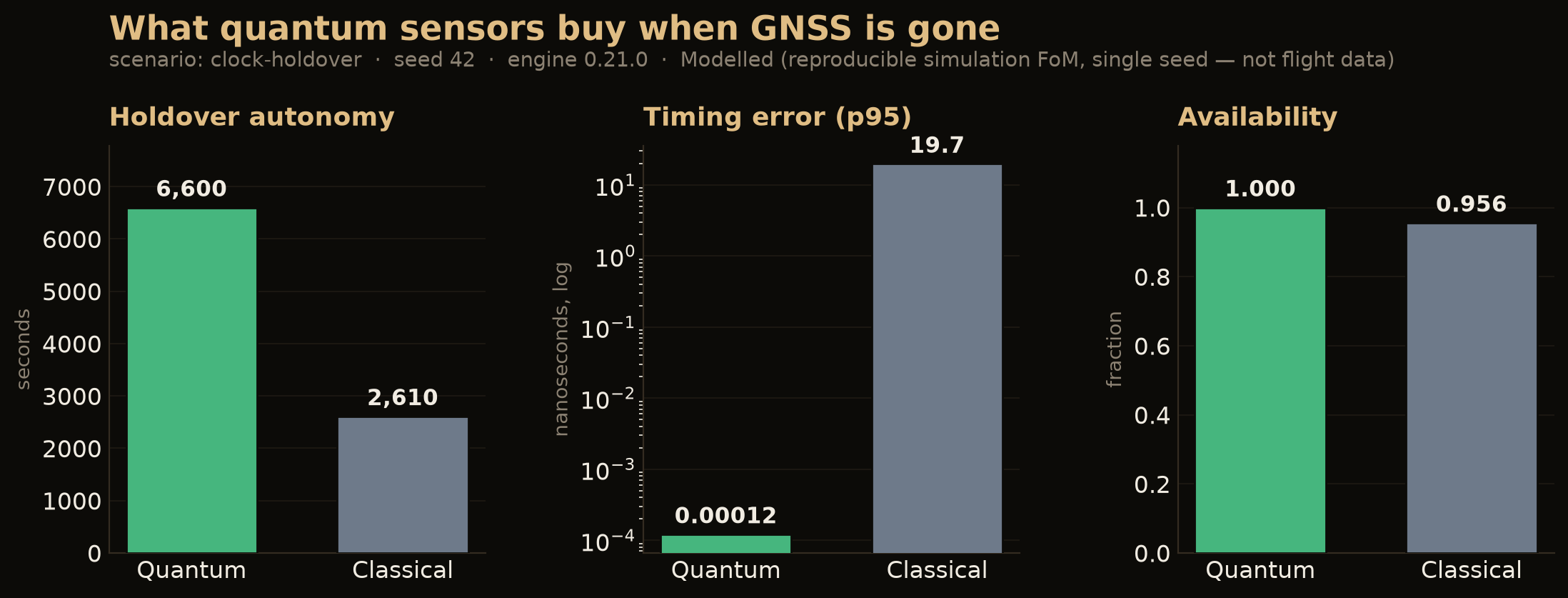
What quantum sensors buy when GNSS is gone — clock-holdover · seed 42 · drawn at engine 0.34.1, and every figure above re-checked against the current engine on each build by tests/published_figures_still_reproduce.rs · SVG
The advantage is outage- and vibration-dependent, with an explicit break-even where classical wins — shown honestly across the technology-readiness ladder (optical-clock figures are ground-demonstrator targets; no strontium optical clock has flown):
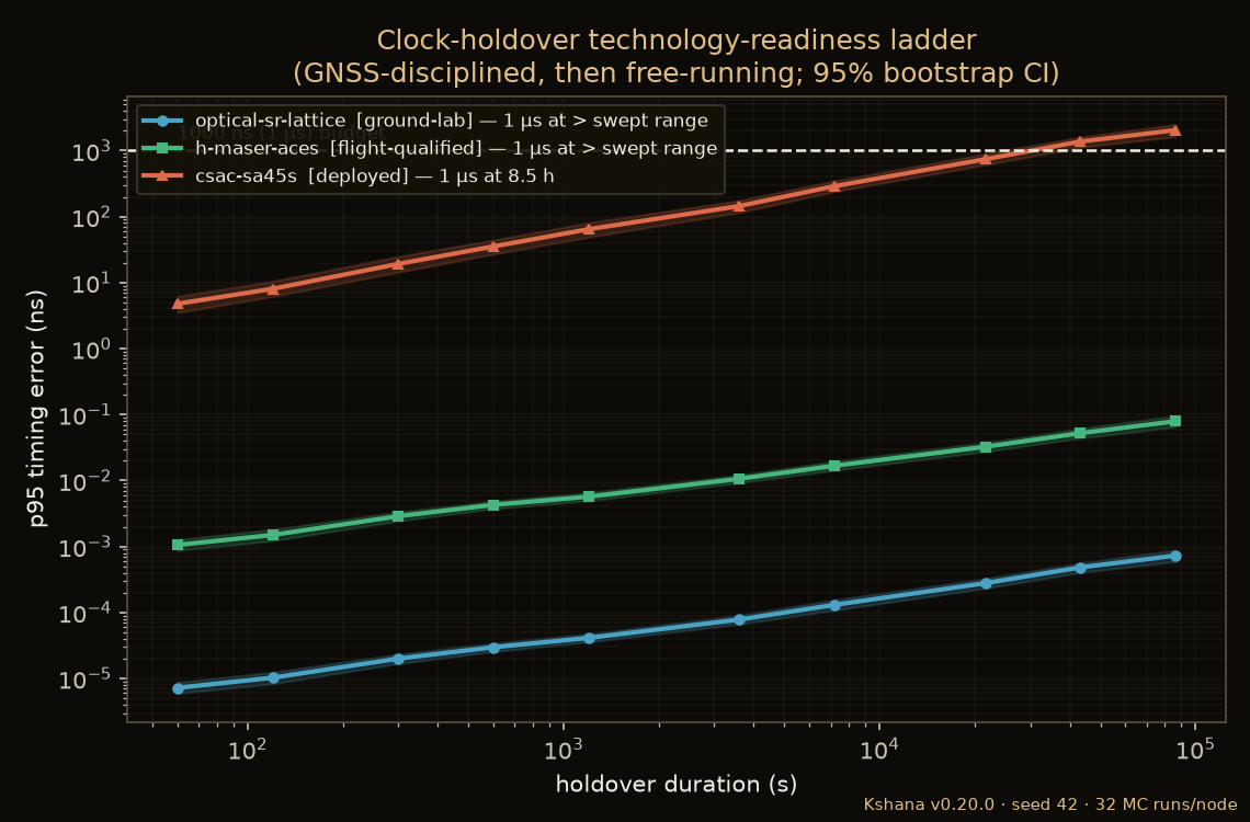
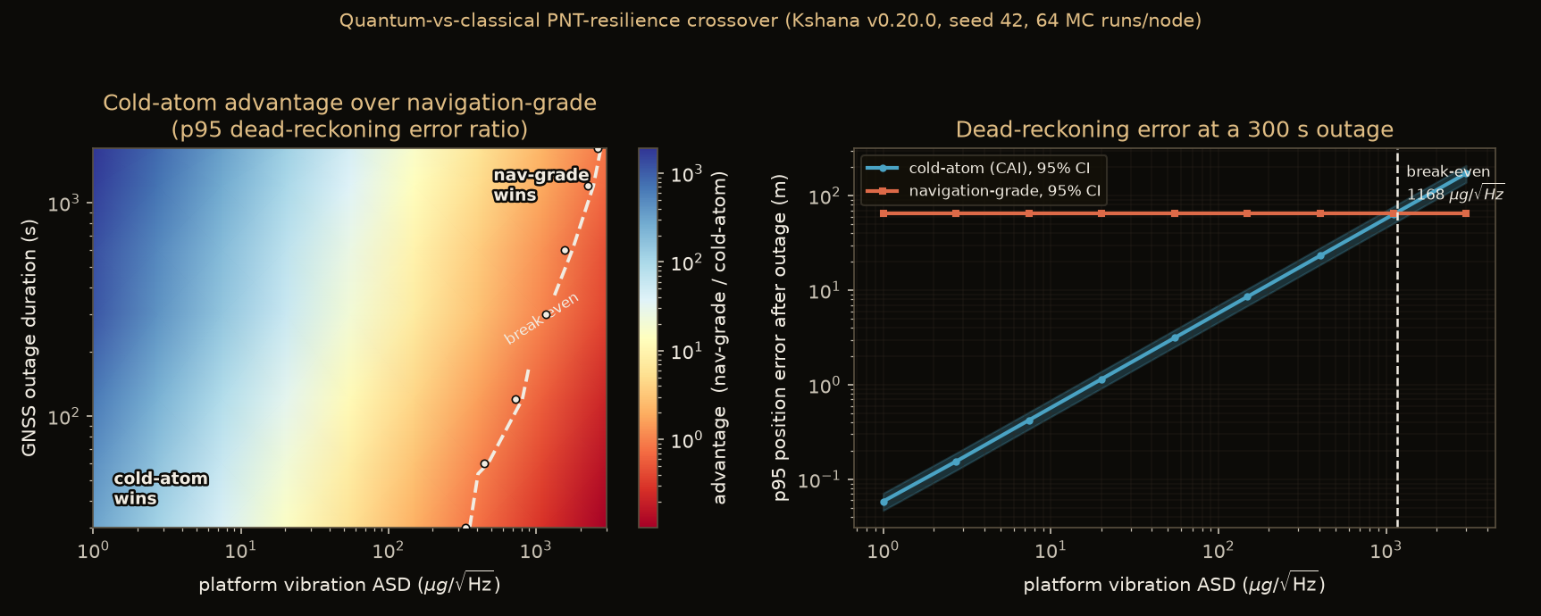
Quantum-vs-classical resilience crossover — clock holdover TRL ladder (top) · inertial advantage map with break-even contour (bottom). Regenerable via cargo run --release --bin crossover_study.
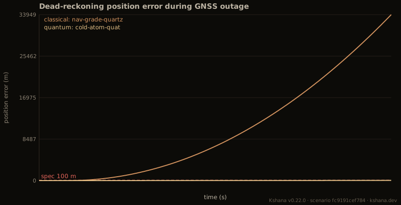
Dead-reckoning position error during a GNSS outage: the quantum sensor (blue)
stays flat near the spec; the classical sensor (red) diverges to tens of kilometres.
Generated by Kshana from scenarios/imu-deadreckoning.toml.
| Pack | Scenario | Quantum | Classical |
|---|---|---|---|
| 1 — Clock holdover | clock-holdover.toml (20 ns spec) | optical clock holds the full outage | CSAC breaches the spec mid-outage |
| 2 — Inertial dead-reckoning | imu-deadreckoning.toml (100 m spec) | cold-atom: ~41 m, holds full outage | nav-grade: breaches in ~350 s → tens of km |
| 3 — Time transfer (optical inter-satellite link) | timetransfer.toml | optical: ~0.3 mm ranging | RF (TWSTFT): ~150 mm ranging |
| 4 — Hybrid fusion (capstone) | hybrid-pnt.toml | full position+timing for the whole outage | position-limited at ~350 s |
The capstone shows the fusion thesis: optical inter-satellite time-transfer keeps even a classical clock locked, isolating the inertial sensor as the classical suite's weak link — i.e. quantum inertial + optical timing together.
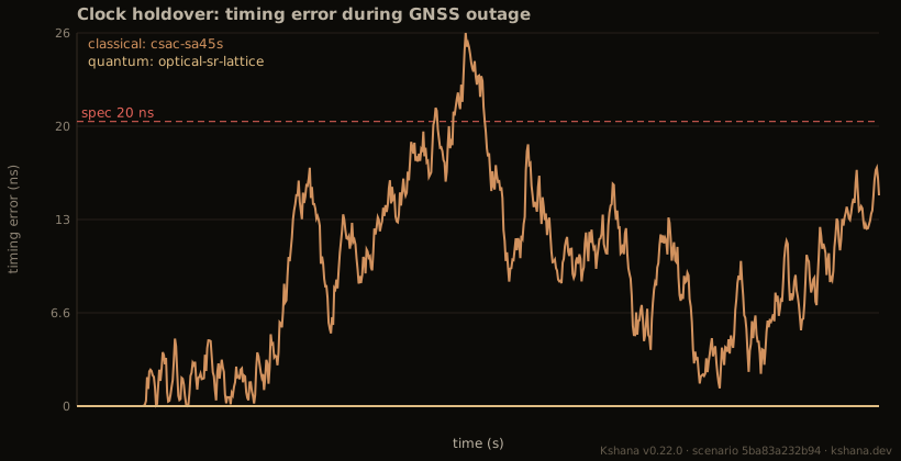
Clock holdover through a GNSS outage: the optical clock (blue) stays inside the
20 ns spec for the full coast; the chip-scale clock (red) breaches it part-way.
Generated by Kshana from scenarios/clock-holdover.toml.
A further scenario, orbit-gnss-challenged.toml, derives GNSS availability from
orbital geometry rather than hand-authored windows: a spacecraft inside the GNSS
shell is propagated against a GPS-like Walker constellation, and the visible-satellite
count (line-of-sight, Earth-occultation, elevation mask) sets the fix state at each
step. Over a day the user is in fix only ~59% of the time; the quantum clock holds a
5 ns timing solution through every gap (availability 1.0), the chip-scale clock
only ~0.83.
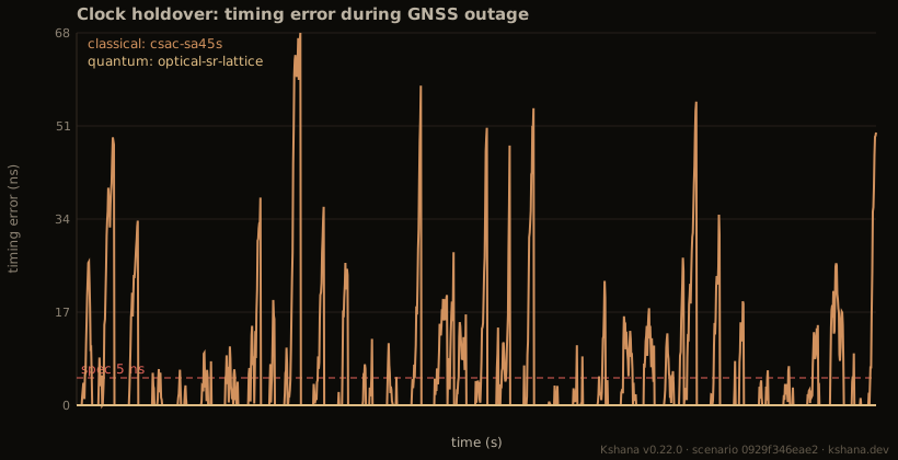
Timing error over a day with GNSS availability derived from orbital geometry: the
visible-satellite count (line-of-sight, Earth-occultation, elevation mask) sets the fix
state at each step, so the clock must coast every gap — the optical clock holds the 5 ns
spec while the chip-scale clock breaches it. Generated by Kshana from
scenarios/orbit-gnss-challenged.toml.
The constellation can also be given as real two-line element sets (TLEs). A full TLE
(line 1 + line 2) is propagated with the full SGP4/SDP4 model — including
atmospheric drag and the deep-space lunar-solar and 12 h / 24 h resonance terms that
matter for ~12 h GNSS orbits — validated against the official AIAA 2006-6753 vectors
to a worst-case ≈ 4 mm. scenarios/orbit-sgp4-gps.toml ships a real Celestrak
gps-ops snapshot of the operational GPS constellation (2021-07-28, 30 satellites)
and requires valid TLE checksums — two-line element sets are open data from the US
Space Force / 18th Space Defense Squadron catalogue, redistributed by Celestrak
(Dr T. S. Kelso, celestrak.org); refresh with
scripts/fetch_tles.sh. A line-2-only block keeps
the analytic two-body propagation (scenarios/orbit-real-tle.toml); the two forms can
be mixed in one constellation. A constellation can equally be built from a block of
RINEX-3 GPS broadcast-ephemeris records — the format a receiver decodes —
propagated by the IS-GPS-200 user algorithm and fed through the same geometry
(scenarios/orbit-rinex.toml).
What it is / is not, in full
What it is / is not
It is: a deterministic, dependency-light engine spanning the PNT stack — orbit geometry, inertial navigation, GNSS/INS fusion, integrity, clocks, and timing. It runs a scenario (often a GNSS outage), evolves calibrated sensor error models through the appropriate estimator, and scores the result against the operational figures of merit — emitting a reproducible JSON (JavaScript Object Notation) result and an SVG chart, from a Rust library, a command-line interface (CLI), a Python extension, an in-browser WebAssembly module, a Model Context Protocol (MCP) server for AI agents, or a JetBrains IDE (integrated development environment) plugin.
It is not: flight hardware, a quantum-payload design, a full GNSS signal receiver, a radio-frequency (RF) signal simulator or hardware-in-the-loop rig, or a certified avionics product — and it does not replace MATLAB/Simulink, STK (Systems Tool Kit) or Orekit